

This study proposes a low-dose CT (LDCT) image denoising technique that integrates a pixel-level non-local self-similarity (NSS) prior with the Non-Local Means (NLM) algorithm. The denoising process is organized into three main stages. In Stage 1, non-local similar pixels are identified to estimate the noise level, followed by the application of the Haar transform with bi-hard thresholding to evaluate local signal intensity and generate a basic denoised image. In Stage 2, the NLM algorithm is applied to refine this preliminary output. Stage 3 involves performing the Haar transform on pixel matrices obtained from both the input image and the NLM-denoised image, applying Wiener filtering, and then executing the inverse Haar transform. Finally, the denoised pixel matrices are aggregated to produce the final restored image. An overview of this complete denoising workflow is illustrated in Fig. 1.
Stage 1: (a) Search for non-local similar pixels
Let the input noisy image be denoted as \(\:y\:\in\:\:{\mathbb{R}}^{h\times\:m}\). The image is divided into a total of N local patches56. Each square patch of size \(\:\sqrt{n}\times\:\sqrt{n}\:\:\)is vectorized into a column vector \(\:{y}_{l,1}\:\in\:\:{\mathbb{R}}^{n}\) for \(\:l=\text{1,2},\dots\:,\:N\). For each patch \(\:{y}_{l,1}\), its\(\:\:m\) most similar patches including itself are identified by computing the Euclidean distance within a sufficiently large search window of size \(\:W\times\:W.\) These mmm patches are then stacked column-wise to form the noisy patch matrix:
$$\:{Y}_{l}=\:\left[{y}_{l,1},\:{y}_{l,2},\dots\:..,{y}_{l,m}\right]\:\in\:\:\:{\mathbb{R}}^{n\times\:m}$$
(6)
To capture pixel-level non-local self-similarity, we analyse each row of \(\:{Y}_{l}\), where each row contains mmm pixels at the same relative location across mmm similar patches. Although patch-level NSS implies some uniformity, variations especially in rare textures or structural details can introduce significant pixel-level discrepancies, leading to artifacts if treated uniformly. To address this, we selectively identify the most consistent rows (i.e., pixels with the highest similarity). For the\(\:\:i\)-th row \(\:{y}_{l}^{i}\in\:\:{\mathbb{R}}^{m}\), the Euclidean distance to the \(\:j\)-th row \(\:{y}_{l}^{i}\left(j=1,\dots\:.,n\right)\) is computed as:
$$\:d_{l}^{{\left( {i,j} \right)}} = \:\left\| {y_{l}^{i} – y_{l}^{j} } \right\|_{2} \:$$
(7)
Naturally, \(\:{d}_{l}^{\left(i,j\right)}\)= 0. Based on this metric, we select\(\:\:q\) rows (where \(\:q\) is a power of 2) that are closest to the reference row \(\:{y}_{l}^{i}\), denoted by:
$$\:\left\{{y}_{l}^{\left({i}_{1}\right)},\:{y}_{l}^{\left({i}_{2}\right)},\:\dots\:\dots\:.,\:{y}_{l}^{\left({i}_{q}\right)}\right\}\:,\:\:\:\:\:\:\text{w}\text{h}\text{e}\text{r}\text{e}\:{i}_{1}=i$$
(8)
These rows are assembled to form a pixel matrix:
$$\:{Y}_{l}^{\left(iq\right)}=\:\left[\left(\begin{array}{ccc}{y}_{l}^{{i}_{1},1}&\:\cdots\:&\:{y}_{l}^{{i}_{1},m}\\\: \vdots &\:\ddots\:&\: \vdots \\\:{y}_{l}^{{i}_{q},1}&\:\cdots\:&\:{y}_{l}^{{i}_{q},m}\end{array}\right)\right]\:\in\:{\mathbb{R}}^{q\times\:m}$$
(9)
Here\(\:,\:q\) represents the number of similar rows (pixels), and \(\:\left\{{i}_{1},\dots\:.,{i}_{q}\right\}\:\subset\:\:\left\{1,\dots\:.,n\right\}\:\). The set of all such matrices \(\:\left\{{Y}_{l}^{\left(iq\right)}\right\}\:\)for all patches \(\:l=1\:,\dots\:,N\) and rows \(\:i=1\:,\dots\:,n\) are used in the subsequent steps for accurate noise level estimation.
Stage 1: (b) noise level Estimation
Accurately estimating the noise level is a crucial step for effective image denoising. We adopt a pixel-level nonlocal self-similarity (NSS) prior for this purpose, which assumes that the selected\(\:\:q\) rows from each patch matrix \(\:{Y}_{l}^{iq}\in\:\:{R}^{q\times\:m}\) contain highly similar pixels and differ primarily due to additive Gaussian noise. Under this assumption, the statistical variation among these pixels can be attributed to noise, allowing us to compute the standard deviation as an estimate of the noise level. For each row \(\:{y}_{li}\) of matrix \(\:{Y}_{l}\), we identify the \(\:q\) most similar rows (including itself), forming the matrix \(\:{Y}_{l}^{iq}\) containing similar pixel values across mmm patches. To quantify the local noise level \(\:{\sigma\:}_{l}\), we compute the pairwise Euclidean distances \(\:{d}_{l}^{{ii}_{t}}\) between the reference row and its \(\:q-1\) most similar rows. Each distance measures the cumulative squared deviation across the mmm corresponding pixel positions.
To convert this cumulative deviation into an average per-pixel estimate, we normalize each squared distance by \(\:m\) (the number of similar patches) and then take the square root, yielding the root-mean-square (RMS) deviation. The final noise level \(\:{\sigma\:}_{l}\) is then obtained by averaging these RMS deviations across all \(\:n\) rows in the patch:
$$\:{\sigma\:}_{l}=\frac{1}{n\left(q-1\right)}\sum\:_{t=2}^{q}\sum\:_{i=1}^{n}\sqrt{\frac{1}{m}}{\left({d}_{l}^{{ii}_{t}}\right)}^{2}\:\:\:$$
(10)
where \(\:\sqrt{1/m}\) term arises from normalizing the squared Euclidean distance between rows (each consisting of mmm pixels) to obtain a per-pixel root-mean-square (RMS) deviation. This normalization ensures that \(\:{\sigma\:}_{l}\:\)estimates the standard deviation of noise at the pixel level, rather than over entire patch vectors. This normalization is important for scale-invariant estimation and aligns with the assumption that noise follows a Gaussian distribution. However, we observe that Eq. (5) performs well in smooth regions but may overestimate noise in structured or textured areas where signal and noise are difficult to separate. To address this, we extend the estimation from local to global by computing the average noise level across all\(\:\:N\) patch groups:
$$\:{\sigma\:}_{g}=\:\frac{1}{N}\sum\:_{l=1}^{N}{\sigma\:}_{l}\:$$
(11)
This global noise level \(\:{\sigma\:}_{g}\) is then used in the subsequent denoising stages to ensure consistency and robustness across varying image regions.
The use of a Gaussian model for noise and the pixel-wise NSS assumption is supported by prior studies57, and the formulation in Eq. (10) offers a computationally simple yet accurate means of estimating noise levels directly from the image data.
Stage 1: (c) Estimation of local signal intensity using Haar transform-based bi-thresholding
In this step, we estimate the local signal intensity from the grouped matrices \(\:{Y}_{l}^{q}\in\:\:{\mathbb{R}}^{q\times\:m}\), where each matrix consists of pixels with similar intensity patterns across non-local patches for each \(\:l=1,…,N\). For simplicity, the pixel index\(\:\:i\) is omitted. A global noise level \(\:\sigma\:\) is first estimated, and the denoising is then performed in the Haar transform domain58. To accomplish this, we employ the lifting Haar wavelet transform (LHWT)59, which is chosen for its computational efficiency, low memory footprint, and adaptability. LHWT is applied to each noisy pixel matrix using two orthogonal transform matrices, \(\:{H}_{l}\:\in\:{\mathbb{R}}^{q\times\:\text{q}}\) and \(\:{H}_{r}\:\in\:{\mathbb{R}}^{m\times\:\text{m}}\), where both\(\:\:q\) and \(\:m\:\)are powers of two. The transformation yields a coefficient matrix \(\:{C}_{l}^{q}\:\in\:{\mathbb{R}}^{q\times\:\text{m}}\)given by:
$$\:{C}_{l}^{q}={H}_{l\:}.\:\:{Y}_{l}^{q}{\:.\:\:H}_{r}$$
(12)
To suppress noise, we apply element-wise hard thresholding to each coefficient \(\:{C}_{l}^{q}\left(i,j\right)\) by retaining only those values exceeding a predefined threshold \(\:\tau\:{\sigma\:}_{g}^{2}\). The resulting thresholded matrix \(\:{\widehat{C}}_{l}^{q}\) is computed as:
$$\:{\widehat{C}}_{l}^{q}=\:{C}_{l}^{q}\circ\:{I}_{\left|{C}_{l}^{q}\right|\:\ge\:\:\tau\:{\sigma\:}_{g}^{2}}\:,\:$$
(13)
Here, ∘ denotes element-wise multiplication and \(\:I\) is the indicator function. According to wavelet theory59, the final two rows of \(\:{C}_{l}^{q}\) (excluding the first column) primarily capture high-frequency components, which often correspond to noise. To further suppress these components, we apply structural hard thresholding by zeroing out all coefficients in these rows, producing the refined matrix \(\:{\stackrel{-}{C}}_{l}^{q}\)
$$\:{\stackrel{-}{C}}_{l}^{q}\left(i,j\right)={\widehat{C}}_{l}^{q}\left(i,j\right)\:\circ\:\:{I}_{if\:i=1,\dots\:..,q-2\:or\:j=1}\:\:$$
(14)
The denoised pixel matrix \(\:{\stackrel{-}{Y}}_{l}^{q}\) is then reconstructed from the thresholded coefficients by applying the inverse LHWT:
$$\:{\stackrel{-}{Y}}_{l}^{q}=\:{H}_{il}\:.\:{\stackrel{-}{C}}_{l}^{q}\left(i,j\right)\:.\:{H}_{ir,}\:\:$$
(15)
where \(\:{H}_{il}\in\:{\mathbb{R}}^{q\times\:\text{q}}\) and \(\:{H}_{ir}\in\:{\mathbb{R}}^{m\times\:\text{m}}\:\)are the corresponding inverse LHWT matrices. The details of both forward and inverse LHWT operations for specific values of \(\:q\) and \(\:m\) are available in56. Finally, all denoised matrices \(\:{\stackrel{-}{Y}}_{l}^{q}\) are aggregated to reconstruct the globally denoised image. The refined coefficients \(\:{\stackrel{-}{C}}_{l}^{q}\:\)represent local signal intensities, which are critical for accurate image restoration. To ensure optimal estimation of these intensities, the LHWT-based bi-hard thresholding is iteratively applied for K cycles.
Stage 2: fast non-local means algorithm
The central objective of this stage is to efficiently compute the similarity weights \(\:w(i,j\)) as defined in Eq. (2), which are critical for the denoising process. To simplify the explanation, we consider a one-dimensional (1D) case, which can be easily extended to higher dimensions. Let the 1D image domain be \(\:{\Omega\:}=\left\{\text{0,1},\dots\:..,n-1\right\}\), where \(\:n\) is the total number of pixels. Given a translation vector \(\:{d}_{x}\), we define a function \(\:{S}_{{d}_{x}}\left(p\right)\) to compute the cumulative squared difference between the denoised image \(\:{\stackrel{-}{Y}}_{l}^{q}\:\)and its shifted version:
$$\:{S}_{{d}_{x}}\left(p\right)=\sum\:_{k=0}^{p}{\left({\stackrel{-}{Y}}_{l}^{q}\left(k\right)-{\stackrel{-}{Y}}_{l}^{q}\left(k+{d}_{x}\right)\right)}^{2}\:\:\:\:\:\:p\in\:{\Omega\:}\:$$
(16)
This function provides a pre-integrated difference measure that significantly accelerates the computation of similarity weights. Since calculating \(\:{S}_{{d}_{x}}\left(p\right)\) requires accessing pixels beyond the image boundaries, symmetric or periodic padding is employed to preserve data consistency and prevent cache overflow during processing. In the 1D scenario, the patch window is defined as \(\:\varDelta\:= \left[\kern-0.15em\left[ { – P, \ldots \:.,P} \right]\kern-0.15em\right]\). To reduce computational complexity, we replace the Gaussian kernel traditionally used for weighting with a constant value, assuming negligible variation. With this simplification, Eq. (2) becomes:
$$\:\text{w}\left(i,j\right)={g}_{h}\left(\sum\:_{{{\updelta\:}}_{x}\in\:{\Delta\:}}{\left({\stackrel{-}{Y}}_{l}^{q}\left(i+{\delta\:}_{x}\right)-{\stackrel{-}{Y}}_{l}^{q}\left(j+{\delta\:}_{x}\right)\right)}^{2}\right)$$
(17)
Here, \(\:{g}_{h}\:\)(⋅) is a non-increasing function that quantifies the similarity between two-pixel neighbourhoods. To optimize further, we set \(\:{d}_{x}=\:j-i\) and \(\:\widehat{p}=i+{{\updelta\:}}_{x}\), enabling a reformulation of the weight expression:
$$\:\text{w}\left(i,j\right)={g}_{h\:}\left(\sum\:_{\widehat{p}=i-\mathsf{P}}^{i+\mathsf{P}}{\left({\stackrel{-}{Y}}_{l}^{q}\left(\widehat{p}\right)-{\stackrel{-}{Y}}_{l}^{q}\left(\widehat{p}+{d}_{x}\right)\right)}^{2}\right)\:$$
(18)
This formulation allows us to compute weights more efficiently by referencing the precomputed \(\:{S}_{{d}_{x}}\)values:
$$\:\stackrel{-}{w}\left(i,j\right)={g}_{h}\left({S}_{{d}_{x}}\left(i+\mathsf{P}\right)-{S}_{{d}_{x}}\left(j-\mathsf{P}\right)\right)\:$$
(19)
Since \(\:{S}_{{d}_{x}}\:\)is known and P is fixed, this computation becomes independent of the patch size, significantly reducing complexity. This key result enables fast and scalable similarity evaluation across large image domains. In general, for \(\:d\)-dimensional images, the approach results in a computational complexity of \(\:O\left({2}^{d}\right)\:,\:\)making it highly efficient compared to conventional formulations, such as that in54, which scale with both patch size and image dimensions. The fast NLM algorithm proceeds as follows: first, all \(\:{S}_{{d}_{x}}\:\)values are computed using Eq. (16); next, the similarity weights are calculated using Eq. (2) through (17); finally, denoising is performed by weighted averaging based on Eq. (1). This process is repeated across all translation vectors within the defined search window.
Stage 3: Wiener filtering for final denoising
The denoised image obtained from Stage 2 serves as a preliminary estimate of the clean image but may still retain residual noise. To refine this result, Stage 3 applies Wiener filtering for enhanced denoising while preserving important structural details. This process leverages soft-thresholding within the Haar transform domain, guided by the previously estimated local signal intensities and global noise level \(\:{\sigma\:}_{g}\). Wiener filtering is applied to the LHWT (Lifting Haar Wavelet Transform) coefficients of the original noisy pixel matrices. The filter adaptively attenuates noise based on local signal-to-noise characteristics. Specifically, for each coefficient \(\:{C}_{l}^{q}\left(i,j\right)\) from Eq. (12), the Wiener-filtered output \(\:{\stackrel{-}{C}}_{l}^{q}\left(i,j\right)\) is computed as:
$$\:{\stackrel{-}{C}}_{l}^{q}\left(i,j\right)=\:\frac{{\left|\stackrel{-}{w}\left(i,j\right)\right|}^{2}}{{\left|\stackrel{-}{w}\left(i,j\right)\right|}^{2}+{\left({\sigma\:}_{g}/2\right)}^{2}}\:\:{C}_{l}^{q}\left(i,j\right)\:$$
(20)
Here, \(\:\stackrel{-}{w}\left(i,j\right)\:\)represents the pixel value obtained from the denoised output of Stage 2 (Eq. 19), and \(\:{\sigma\:}_{g}\) denotes the global noise level. Notably, this stage requires both the original noisy image and its denoised counterpart from Stage 2 to effectively compute the filtering coefficients. To apply the Wiener filter, the matrices of non-local similar pixels from both the input and the denoised image are first transformed using LHWT. Wiener filtering is then applied in the transform domain using Eq. (20), and the filtered coefficients are subsequently transformed back into the spatial domain via inverse LHWT, yielding the refined denoised matrix \(\:{\stackrel{-}{Y}}_{l}^{q}\). Finally, all such filtered matrices \(\:{\stackrel{-}{Y}}_{l}^{q}\:\)are aggregated across the image to produce the final, high-quality denoised output. This stage enhances detail preservation and significantly reduces remaining noise offering a more accurate restoration of the latent clean image.
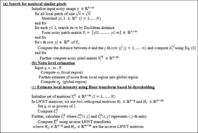
Algorithm 1. Pseudocode for Stage 1.
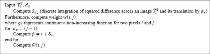
Algorithm 2. Pseudocode for Stage 2.

Algorithm 3. Pseudocode for Stage 3.
link