To evaluate our proposal, we considered three well-known and publicly available healthcare datasets containing data on diabetes patients, pneumonia, and NIH Chest X-ray images, respectively. We have made the evaluation codes available.Footnote 1
We conducted a comprehensive evaluation using widely adopted fairness metrics and explainability techniques to evaluate the efficacy of ECGL in enhancing the overall fairness and explainability of machine learning models. We evaluated the efficacy of our proposed ECGL in (i) mitigating biases that may lead to discriminatory outcomes and (ii) enhancing transparency into the model’s decision-making process.
Evaluation
We utilized two prominent techniques to interpret and explain the predictions of models: SHAP [47] and GradCAM [48]. We employed SHAP (SHapley Additive exPlanations) values to interpret the importance of features in the models’ predictions (first experiment with the diabetes dataset). SHAP values provide a measure of how much each feature contributes to the difference between a prediction and the average prediction of the model. Therefore, SHAP values can reveal the most influential features in a model’s prediction, feature interaction, and global and local explanations.
For the second experiment with the pneumonia X-ray image dataset, we used GradCAM (Gradient-weighted Class Activation Mapping) to visualize the regions of the images that the model focused on when making predictions. GradCAM generates heatmaps that highlight the areas of the image that contribute most to the model’s classification. These heatmaps offer insights into how the models are making decisions, potentially revealing biases or limitations. By analyzing the regions highlighted by the heatmaps, we can identify which features (e.g., lung nodules, anatomical structures) are most important for the models’ predictions.
The utilized metrics on fairness are presented in [33, 34, 49] and reported below. The insights derived from fairness metrics can effectively guide the model development process toward mitigating biases. In our experiments, dealing with medical datasets, we considered the Equalized Odds Difference (EOD) and Ratio (EOR) as the fairness metric. This metric evaluates the difference and ratio of the true positive and false positive rates between protected groups, respectively. A difference value of 0 and a ratio closer to 1 suggest that the model is equally likely to classify individuals from different groups correctly or incorrectly. EOD and EOR focus on the fairness of the model’s predictions rather than the overall outcomes, ensuring that the conditional probability of a positive outcome given a positive or negative prediction is equal across different demographic groups. Moreover, equalized odds does not enforce the same positive prediction rates across different groups, allowing it to better reflect differences in base rates of outcomes. This is particularly important in domains where certain conditions may be more prevalent in specific demographic groups.
Additionally, we have utilized common metrics, including Area Under Curve (AUC) and Accuracy to measure the model’s performance. Overall, higher AUC and Accuracy values indicate a more accurate model, while lower EOD and higher EOR represent a fairer model.
Experimental settings
To evaluate our proposal, we considered three well-known and publicly available healthcare datasets containing data on diabetes patients and pneumonia and NIH Chest X-ray images, respectively. The experiments on diabetes and pneumonia datasets have been conducted on a system with 2 Intel Xeon virtual CPUs and 12 GB of RAM, using the Python programming language and TensorFlow library. The experiment on the NIH Chest X-ray images was conducted using 2 T4 GPUs, 30 GB of RAM, and 16 GB of GPU RAM. “Fairlearn” and “SHAP” libraries have been used for fairness and explainability evaluation purposes, respectively. The GradCAM visualization has been implemented by the authors using the “Keras” library. We have also used the “Scikit-learn” library for data preprocessing and standardization.
Experiment I: diabetes dataset
The diabetes datasetFootnote 2 is a widely used benchmark in the healthcare domain. This dataset comprises 768 instances with eight attributes, including gender, body mass index (BMI), blood pressure, skin thickness, insulin level, glucose level, and diabetes pedigree function. The target variable is a binary class indicating the presence or absence of diabetes. We evaluated the performance of the proposed model across a range of different metrics, including EOD, EOR, Accuracy, and AUC.
Model selection
The model architecture of the examined diabetes deep learning network is illustrated in Fig. 1. We utilized a sequential neural network, consisting of three dense layers with decreasing units (128 \(\rightarrow\) 64 \(\rightarrow\) 32), interspersed with dropout layers to prevent overfitting. The final layer has two output units with a softmax activation function, producing probabilities for the two classes, referring to the positive or negative case of diabetes.
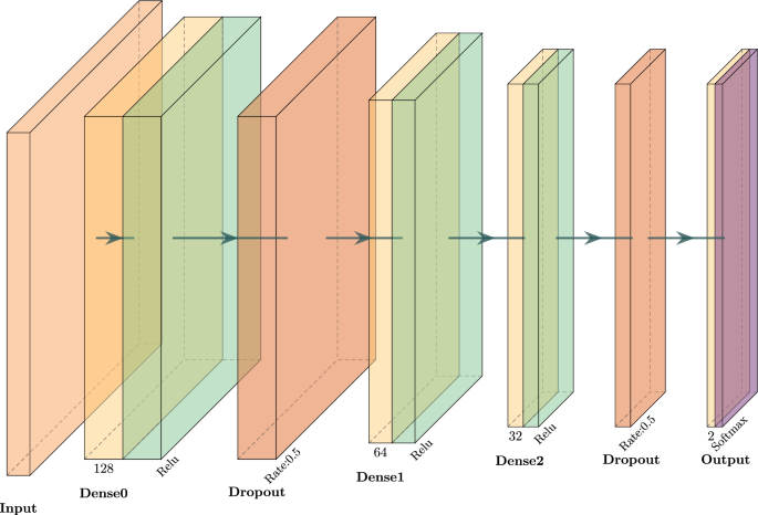
The architecture of the neural network was utilized for the experiment on the diabetes dataset
As for the training, we used the sparse categorical cross-entropy loss function and the “Adam” optimizer. The model has been trained considering 100 epochs in total, with early stopping applied to avoid the potential of overfitting.
Explanation constraints
To effectively define explanation constraints in our model, we conducted a comprehensive analysis of the dataset and leveraged expert domain knowledge. This analysis allowed us to identify the relevant ranges and the correlations of data features with the likelihood of a positive diabetes diagnosis. We identified the potential probability of positive and negative diabetes cases corresponding to the specified feature ranges reported in Table 1. We defined the corresponding constraints and used them to refine and guide the model’s predictions towards classification labels aligning with the determined probabilities. Noteworthy, we consider the normalized values of these conditions to better align with loss values while training the model.
In particular, each condition in Table 1 specifies a corresponding constraint violation function \(g(\theta)\), which evaluates the inconsistency between the model predictions and expert probabilities under a given range of a feature. For a sample whose features lay in a specified range (say Glucose > 170), this constraint violation is assessed concerning the probabilities output by the model. For instance, should domain knowledge indicate a high degree (e.g., 0.84) of a positive diagnosis for the high glucose class, then this constraint term penalizes the model when it predicts low probabilities for this class. The violation itself is expressed as a smooth and differentiable function of model outputs, which measures the model’s failure to conform with the expert knowledge. Such a formulation easily lends itself to gradient-based optimization in the Augmented Lagrangian framework.
The set of constraints in Experiment I is all defined over closed intervals or threshold-based conditions for individual features; hence, they define convex feasible regions in the input space. In Table 1, the classification of each condition with respect to convexity is presented. This makes it compatible with convex constraint optimization techniques; however, our framework remains applicable even in non-convex scenarios because of its iterative penalty-based scheme.
Results and discussion
The Base model was trained to optimize the output accuracy without any explanation constraints. Table 2 compares the base network with ECGL variants that impose explanation constraints on individual features or on all features simultaneously. The All-constraints model achieves the highest accuracy (0.7857, +3.89% over Base Model) but does not improve fairness (EOD = 0.3399, identical to the Base model; EOR = 0.3174 vs. 0.3265). In contrast, several single-feature variants provide meaningful fairness gains: the Pregnancies-only model reduces EOD by 43% (0.1931) and raises AUC by 4.84% (0.7646). Overall, imposing carefully chosen explanation constraints can lower bias while preserving—or slightly improving—predictive performance; combining all constraints maximizes accuracy at the cost of fairness.
Explainability analysis by using the SHAP values is presented in Table 3. As shown in Table 3, the feature importance values generally experience an increase when the associated explanation constraints are applied during model training. For instance, integrating the constraint associated with Pregnancies led to an approximate 9.6% rise in the importance of this feature in the model’s final prediction. Similarly, several features, such as Skin Thickness and Insulin, exhibited substantial increases in their SHAP importance values. However, a few features, such as BMI and DPF, showed a slight decrease. Moreover, by combining all constraints, the All Constraints model achieves an overall improvement in feature importance alignment compared to the Base Model, supporting the effectiveness of ECGL in steering the model towards clinically relevant explanations.
SHAP values can also help identify feature interactions, which may be crucial for understanding the model’s behavior. This means that the constraints, including one feature, may also affect how the model adheres to another one. As an example, applying constraints associated with BMI indicates massive improvements across almost all constraints (+93.5% to +234.9%). This suggests that BMI could be considered a highly sensitive parameter to constraints with a critical role in predictions. The Insulin under the Diabetes Pedigree Function (DPF) constraint shows the highest value in the table. BMI and Insulin might be seen as the most “constraint-sensitive” features, since the gains are larger compared to other constraints.
Figure 2 presents SHAP summary plots for the Base model and the proposed ECGL (All Constraint model), which provide a visual representation of the feature’s contribution to the prediction. The color and size of the dots in SHAP summary plots represent the feature’s contribution, while their position (being positive or negative) indicates whether the feature increases or decreases the prediction outcome. In Fig. 2(a) and 2(b), the Base model highlights Glucose and BMI as the most influential features, followed by DPF. Features like Pregnancies, Blood Pressure, Insulin, and Skin Thickness show relatively lower importance. However, the All Constraint model demonstrates a shift in feature importance. While Glucose and BMI remain the most significant features, the importance of Insulin has increased significantly due to the integration of explanation constraints. For instance, the Base model assigns an importance value close to 0 or negative for Insulin, whereas the All Constraint model shows a larger range with more positive and extreme values. Similarly, the features Pregnancies, Blood Pressure, and Skin Thickness exhibit increased importance, indicating that the constraints effectively guide the model to focus on these relevant features.
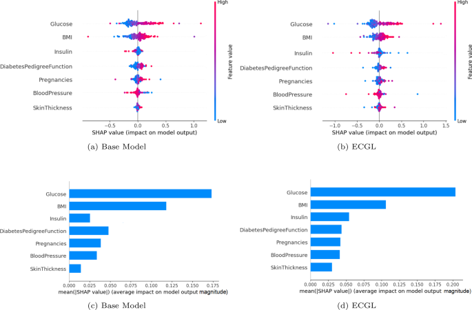
SHAP value evaluation of the base model and ECGL (constraint model). (a) base Model. (b) ECGL. (c) base Model. (d) ECGL
Figures 2(c) and 2(d) illustrate the mean absolute SHAP values for different features, highlighting their relative importance in predicting the target variable for the Base model and the All Constraint model. These plots show that applying constraints has slightly changed the overall feature importance. While Glucose remains the most influential feature, the importance of other features has increased, indicating that the constraints have guided the model to focus more on these features. For example, the importance value of Glucose increased from 0.175 in the Base model to 0.20 in the All Constraint model. Additionally, the constraints had a significant effect on features such as Insulin, Pregnancies, and Skin Thickness, which were not utilized properly in the Base model. This means that the constraints enhanced the model’s learning process, allowing it to better capture the relevance of these features, resulting in improved predictions and interpretations.
Experiment II: pneumonia X-ray images
In this section, we explore the fairness and explainability performance of the proposed ECGL on the pneumonia classification task, using an X-ray image dataset.Footnote 3 This dataset contains 30,000 frontal-view chest radiographs from the 112,000-image public National Institutes of Health (NIH). We employed GradCAM to gain insights into the model’s decision-making process, enabling us to understand the rationale behind its predictions and identify the improvements gained by applying explanation-guided learning on the model.
Model selection
The overall architecture of the model for Experiment II is presented in Fig. 3. Considering the image data, we utilized 2D convolutional layers with the ReLU activation function, accompanied by two max pooling layers with a kernel size of 2. The model employs three output layers with a variety of sizes to predict different features. The primary task output is responsible for predicting the main classification labels, meaning pneumonia classification. The model also yields two more outputs, used to integrate the gender-based and bounding box-based explanations into the model and to guide the model towards predictions more aligned with these constraints. Moreover, the bounding box-based explanation layer predicts the information that can be used to explain the model’s focus on specific regions of the input X-ray image, which increased the model’s transparency regarding the decision-making process and the explainability of the final predictions.
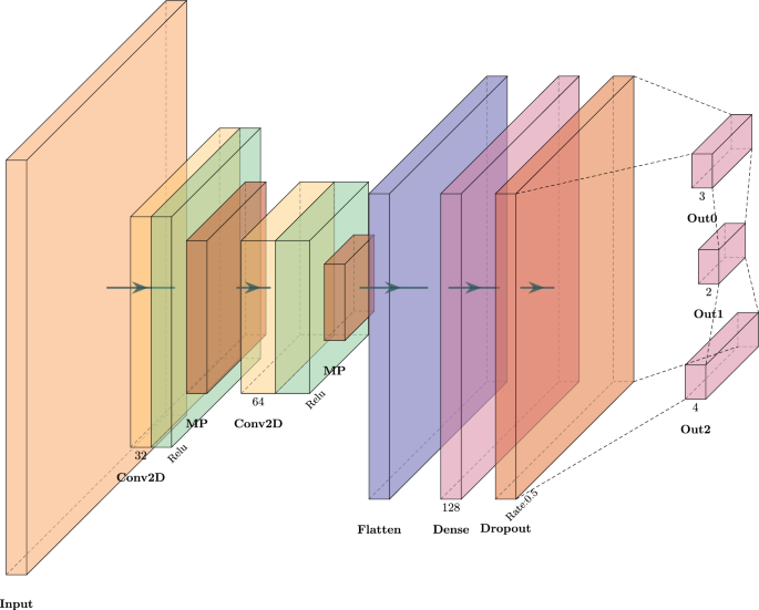
Architecture of the model to evaluate the performance of the proposed ECGL and base model on pneumonia X-ray image classification
Each sample was converted to a 3-channel RGB image with a size of 128 by stacking the original image three times along the last axis while ensuring the image remains clear with anti_aliasing enabled. Then, the data were split into training and test data, considering an 80%-20% ratio for training and validation, respectively. The Base model was trained without any explanation constraints, while for the ECGL model, the explanation constraints were defined and taken into account. Both ECGL and base models were trained for 30 epochs, using 2000 X-ray image samples of the pneumonia dataset, using the Adam optimizer, and sparse categorical cross-entropy and mean absolute error as loss functions for label and bounding-box classification and gender prediction, respectively.
Explanation constraints
To integrate fairness and explainability, we incorporated two primary constraints, including gender-based and bounding box-based constraints. By imposinga gender-based explanation, we aimed to mitigate potential gender bias in our model’s predictions. These explanation constraints are designed to ensure that the model’s outputs are not systematically biased towards or against specific genders. Moreover, the bounding box-based explanation aims to enhance the explainability of our model’s predictions. These explanation constraints are intended to guide the model to focus on relevant regions of the input data, providing insights into the factors that influence its decisions.
Results and discussion
Table 4 presents a comparative analysis of the Base and ECGL models in terms of fairness, accuracy, and AUC. The overall performance of the models reveals that both models demonstrate comparable levels of overall accuracy of 87%, suggesting that the constraints imposed on the ECGL model did not significantly compromise its predictive power. By contrast, the Base model could achieve a slightly higher AUC value, with a relatively small difference of about 4%, while the ECGL model exhibits relatively high performance in mitigating biases and disparities.
Evaluating the EOD and EOR values demonstrates slightly different results. While the Base Model achieves a 3% lower EOD compared to the ECGL Model, the ECGL Model exhibits a noticeable 13% improvement in EOR. As these metrics assess whether the model’s predictions are equally distributed across different groups, the results suggest that the ECGL-enhanced model achieves greater uniformity and fairness in its predictive performance when guided by explanation constraints.
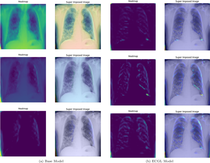
Figures 4 and 5 depict the GradCAM Heatmaps and Superimposed X-ray images of correctly and incorrectly predicted pneumonia instances, respectively. The areas in images that are highlighted in color represent the regions that the model deemed most important for its decision. Moreover, the overlay of the heatmaps on the original X-ray images provides valuable information, allowing us to assess whether the models are focusing on relevant features. The superimposed images refer to the original images combined with the heatmaps, providing a more comprehensible visual representation of the focused regions. The illustrated heatmaps depict three classification outputs corresponding to the labels 0, 1, and 2, arranged from top to bottom, respectively. Label 0 indicates “No Lung Opacity,” which refers to patients without diagnosed pneumonia. The other labels, 1 and 2, on the other hand, signify Lung Opacity and the presence of fuzzy white clouds in the lungs, associated with pneumonia.
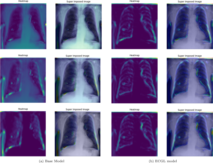
GradCAM Heatmaps and superimposed images of the (a) base model and (b) ECGL model for correctly labeled instances. The illustrated heatmaps correspond to GradCAM visualizations for labels 0 (normal), 1 (pneumonia present), and 2 (pneumonia absent, abnormalities exist), arranged from top to bottom, respectively. (a) base Model. (b) ECGL model
GradCAM Heatmaps and superimposed images of the (a) base model and (b) ECGL model for incorrectly labeled instances. The illustrated heatmaps correspond to GradCAM visualizations for labels 0 (normal), 1 (pneumonia present), and 2 (pneumonia absent, abnormalities exist), arranged from top to bottom, respectively. (a) base Model. (b) ECGL model
Likewise, Figs. 6 and 7 compare the proposed ECGL model and the Base model in terms of explainability by using GradCAM heatmaps. While both models generally seem to be focusing on similar areas (central region) of the chest X-rays, the color intensity in the heatmaps and superimposed images obtained from the ECGL model clearly shows a greater emphasis on certain regions that are related to the respiratory system and pneumonia disease. As it can be seen in Fig. 4(a) and 4(b) (correctly labeled instances), the highlighted regions of the Base model are more blurred, hazy, and spread out across the image, suggesting that the model’s decisions are less interpretable and apparent to the experts. Whereas the proposed ECGL model presents more focused and localized highlighted regions, showing that the model is primarily relying on specific areas of the image, relating to the particular region attacked by the disease, to make its prediction. The ECGL model makes it easier to understand the model’s reasoning and therefore presents more explainability. In addition, the ECGL model produces a more concentrated heatmap, indicating more confidence in prediction.
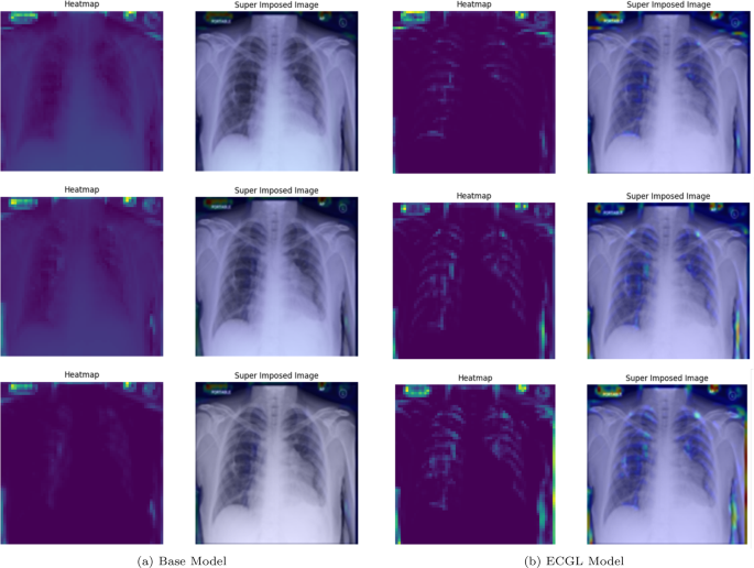
GradCAM Heatmaps (left column) and Superimposed images (right column) of the (a) Base model and (b) ECGL model for correctly labeled instances. The illustrated heatmaps correspond to GradCAM visualizations for labels 0 (normal), 1 (pneumonia present), and 2 (pneumonia absent, abnormalities exist), arranged from top to bottom, respectively
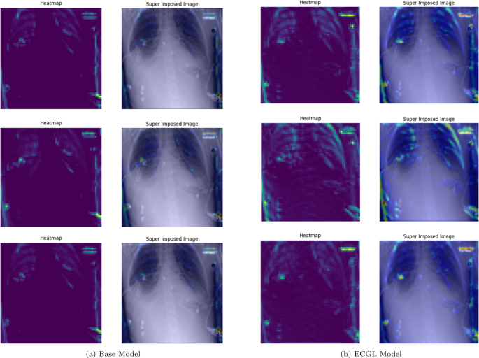
GradCAM Heatmaps (left column) and Superimposed images (right column) of the (a) Base model and (b) ECGL model for incorrectly labeled instances. The illustrated heatmaps correspond to GradCAM visualizations for labels 0 (normal), 1 (pneumonia present), and 2 (pneumonia absent, abnormalities exist), arranged from top to bottom, respectively
Moreover, in spite of both models’ similar performance illustrated in Fig. 5(a) and 5(b), the GradCAM visualizations clearly demonstrate noticeable differences. The Base model resulted in a more scattered visualization that may not correspond to the actual pathology. This indicates that the Base model’s prediction can be based on irrelevant features and not focused on the main required regions. The proposedECGL model, on the other hand, highlighted regions that are more relevant to the considered medical condition, suggesting that the constraints have helped the model focus on more meaningful features.
Unlike the Based model, the ECGL model’s heatmap for the incorrect prediction is more localized, highlighting a specific region in the lung. The overlay shows that there is indeed an abnormality in this area, but it could have been insufficient to confidently classify the image, which resulted in an incorrect final prediction. While such false predictions highlight the complexity of the task, the findings suggest that adding the constraints and guiding the model with domain-specific explanations through proposed ECGL can enhance the model’s explainability even when overall accuracy remains quite the same. Using such explainability, the experts can better identify the model’s deficiencies and limitations, leading to efficient mitigation of them.
A bounding box (BBOX) is a rectangular region that is commonly used to localize (highlight) the interest area. Figure 8 illustrates the BBOX of some pneumonia disease instances predicted by the proposed ECGL model. The red box refers to the ground truth BBOX stated for the X-ray image, and the blue box demonstrates the predicted box by the ECGL model. It is important to note that the Base model cannot generate BBOX due to the lack of explanation constraints required for BBOX prediction.
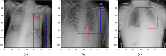
Ground truth (red) and predicted (blue) BBOX regions in X-ray images: (a) and (b) represent the samples where the model predicts an incorrect label, while (c) corresponds to the case of the correct prediction
Looking at Fig. 8(a) and 8(b), it is evident that the proposed ECGL correctly predicted the BBOX, aligning with the true box, even though the model estimated a larger area. This points out that considering the BBOX constraints in the model as integrated explanation constraints is effective in highlighting the attention to more relevant regions. Figure 8(c) presents a case where the predicted BBOX is partially within the lung area and may highlight the need for more refined BBOX constraints to better capture the spatial extent of pneumonia.
ECGL seems promising; however, it also has many limitations. First, we’ve only tried it on three datasets-one for diabetes numbers and two for chest x-ray images. As a result, we don’t yet know how it will behave with data from other hospitals or patient groups. Second, the “explanation rules” that steer the model aren’t produced automatically; they have to be written by clinicians using their know-how plus SHAP plots, and that can be slow and error-prone. Automated methods for discovering constraints could be the theme of future research towards improving scalability. For example, through multi-center data to infer constraints using techniques such as meta-learning, or through unsupervised approaches to detect consistent patterns in model explanations that can, in turn, be formalized as constraints. Third, we looked at fairness for just one binary trait (male vs. female) and one fairness metric (equalized odds). Real-world bias is messier than that. Fourth, the quality of ECGLs explanations is tied to Grad-CAM and SHAP; if those tools point in the wrong direction, the constraints can too. Finally, training with extra fairness-and-explanation losses takes more computational resources and a bit of extra hyperparameter tuning. All of these gaps give us a clear to-do list for the next round of work.
Experiment III: NIH chest X-ray images
We assess the performance of our proposed ECG model with an evaluation on the NIH Chest X-ray dataset.Footnote 4 This is a large-scale anonymized collection of 112,120 frontal views of chest X-ray images labeled via NLP techniques from radiology reports across 14 thoracic disease categories. From this dataset, we have created a balanced subset for a multi-label classification with at least 700 positive samples per class, where we obtain 8,307 training images, 4,973 validation images, and 7,156 test images. Each image is resized to 128 × 128 pixels and normalized to [0, 1]. Horizontal flips, brightness, and contrast perturbations are used for image augmentation in training. Gender is included as an auxiliary label to perform fairness analysis. In order to conduct a fairness assessment on demographic groups, especially the case with gender, we will present multiple group fairness metrics: Demographic Parity Difference (DPD), Demographic Parity Ratio (DPR), Equalized Odds Difference (EOD), Equalized Odds Ratio (EOR), and Statistical Parity Difference (SPD). These metrics assess the disparities concerning model decision outputs and are computed across all the disease labels in the multi-label setting.
Model selection
The architecture of the model has been given in Fig. 9. The architecture has a sequential arrangement of four convolutional blocks, each containing one 2D convolutional layer with ReLU activation, batch normalization, and max pooling. The number of filters in the end convolution outputs gradually increases in powers of 2, namely, 32, 64, 128, and 256. This allows the model to extract more and more abstract spatial characteristics of inputs from NIH chest X-ray images. The output generated by the last convolutional layer is passed through a global average pooling layer before going through dropout (at a dropout rate of 0.5) to deal with overfitting. This is then flattened and fully connected to a dense output line with 512 neurons and L2 regularization prior to a last output layer containing sigmoid-activated neurons, indicating the multi-label classification of diseases. This addresses fairness at this level by adding constraints of explanation based on gender, which causes the model to give similar feature attributions for both genders, reducing demographic bias within the learned representations and predictions. Finally, the model is trained with a batch size of 128 and for 20 epochs.
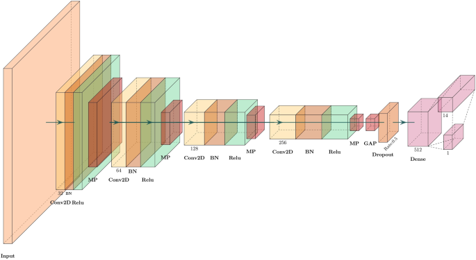
Architecture of the model to evaluate the performance of the proposed ECGL and base model on NIH X-ray multi-label image classification
Explanation constraints
Similar to experiment II, we introduced a gender-based explanation bias as one of the constraints to reduce possible gender bias in model predictions. Such a constraint would ensure that the predictions produced by the model are not systematically affected by gender, promoting equal treatment with respect to demographic groups. By enforcing the same gender-based explanation consistency, we guide the model to align certain attribution patterns between genders, thereby lowering the likelihood of any biased feature attributions arising in its decision-making processes.
Results and discussions
Experimental results on the NIH Chest X-ray dataset are shown in Table 5, while Table 6 reports a detailed comparison between our proposed ECGL model and the baseline CNN model in predictive performance and fairness across demographic groups. With respect to classification performances, both models attain identical validation and testing accuracy (0.8805 and 0.7130, respectively). This means that including explanation constraints in ECGL does not harm classification accuracy. Nevertheless, AUC scores reveal that ECGL has a slightly lower micro-AUC (0.6737 vs. 0.7006) but a marginally better macro-AUC (0.6208 vs. 0.6202). This small increase in macro-AUC may indicate more equitable performance amongst disease classes, especially for rarer conditions, which is one of the more desirable qualities for multi-labels in medical diagnosis.
The major strength of the ECGL lies in the fairness metrics. For most disease types, the ECGL model shows a significant improvement in DPD, EOD, and SPD. For example, the ECGL reduced the EOD for cardiomegaly from 0.11 to 0.03 (73% improvement) and enhanced the EOR by nearly 19%. The same applies to Pneumonia and Pleural Thickness, where ECGL performs well in reducing demographic disparities across various fairness metrics. There are cases where classes have improved or degraded to extremes. For instance, Mass and Nodule have very high drops in SPD, meaning that there has been a large change in the predicted positive rates between gender groups. However, the sign flip in SPD from positive to negative in these classes can be interpreted to mean that fairness improved in one view but was perhaps overcompensated. For Hernia, while DPD and SPD improved, the EOR becomes undefined due to an original zero denominator in the base model, indicating instability in fairness metrics for extremely underrepresented classes. Importantly, some diseases (Consolidation, Edema, Effusion, Infiltration, Pneumonia, Pneumothorax) have seen ECGL reducing fairness gaps or making EOR more balanced. This shows that the model is robust at addressing gender inequalities, presumably across medical model decisions. These results demonstrate that explanation-based fairness constraints can help the model easily engage in fair behavior, especially in predicting cases that might be biased toward some demographic attributes such as gender. In all, ECGL model successfully balances fairness and accuracy, most particularly by making the same level of achievement as the base model while ensuring significant improvements in demographic fairness. This gives credence to the view that integrating explanations as a constraint indeed can work as additional regularization for fairer decision-making in medical imaging applications entailing high stakes, such as multi-labels.
Computational overhead analysis
Table 7 compares the average training time per epoch of the proposed ECGL method against the base model for the three different dataset-and-machinery configurations: CPU-based training for the Diabetes and Pneumonia X-ray datasets, and GPU-based training for the NIH Chest X-ray dataset. Thus, since ECGL imposes explanation penalties according to the Augmented Lagrangian method, its complexity mainly impacts the training stage; average epoch time becomes a relevant measure of the overhead.
The results showed that ECGL incurs additional computational costs compared to the base models in all datasets and hardware configurations. On the rather small Diabetes dataset, using CPU, ECGL increased the average epoch duration from 0.84 seconds to 3.40 seconds, thus increasing the training time by approximately fourfold. This larger relative overhead can be laid against the extra efforts required for computing constraint penalties, updating the Lagrange multipliers, and integrating explanation guidance within each training iteration. All of which form a larger fraction of the total computation being performed on smaller models and smaller datasets. In contrast, the overhead appears less for the Pneumonia X-ray dataset (also CPU-based); average epoch time goes up from 78.85 seconds to 84.64 seconds increase of about 7%. This more modest relative increase reflects that the base training cost for the deeper CNN model has a major role in defining the total training time, thus subsidizing the additional cost of ECGL constraints. Finally, on the NIH Chest X-ray dataset being trained on a GPU, which is a large-scale and more complex scenario, the average epoch time changes negligibly from 405.36 seconds (base) to 409.82 seconds (ECGL), representing less than a 2% increase. This observation shows that in very large deep learning settings that already have a substantial baseline training cost, the extra overhead imposed by the explanation constraints and augmented Lagrangian updates is very small and practically negligible.
The findings say that although relatively measurable computational overhead is introduced by ECGL, with respect to the model and dataset complexity, its relative cost decreases. Such behavior argues for the scalability and efficiency of ECGL for large-scale medical imaging tasks in real-world expectations, wherein the marginal cost is more than compensated by improvements in fairness and explainability. An increase in training time by a small percentage is a worthy trade-off when you take into account the advantages offered by combining domain knowledge with explanation constraints that lead to the generation of trustworthy and equitable models.
Limitations
Although the ECGL framework proposal constitutes promising advances in the incorporation of explanation constraints for fairness and interpretability for a spectrum of datasets, some limitations are also present. First, the experimental evaluation is at present limited to only three datasets while looking primarily at gender as the protected attribute. This can restrict the generalizability of the results to other domains, and thereby, protected groups like race or age is to be addressed in future work. Another point is that while ECGL is able to scale to larger models and datasets with reasonable computational cost, in some extreme large-scale scenarios or resource-constrained environments, the complexity resulting from the augmented Lagrangian methods can be a bottleneck. In particular, the iterative updates of multipliers and penalties. An in-depth inquiry into the computational efficiency and potential optimization methods remains an untapped venue for research.
Thirdly, the explanation constraints in ECGL require a degree of expert knowledge in defining pertinent conditions, which may prevent the scalability and applicability of the method in settings where such input from domain experts is not available. Future works may look into automated or data-driven methods to learn constraints to weaken the need for manual annotation. Finally, the current study concentrates on comparisons against baselines without contrasting with any state-of-the-art fairness and interpretability methods-including adversarial debiasing or alternative explanation frameworks. Extensions on comparisons will be critical to position ECGL firmly within a more extensive scope of methods for explainable and fair AI rigorously. By explicitly acknowledging these limitations, we aim to provide future research directions concerning making explanation-constrained learning frameworks more robust, much more applicable, and much more efficient.
link

